
SageModeler Offers Two System Modeling Approaches
From Earth’s systems to ecosystems to systems in our human bodies, the world is made of interconnected components. Using computational models to represent complex systems can greatly enhance our understanding of how systems work. Students can test their understanding of a system’s complexity by sketching its structure, defining the connections within it, and running the model to see if system outputs match the real world. By comparing a model’s output to observations from the real world, students can iteratively revise both their conceptual models and computational models. SageModeler offers two approaches to computational system modeling that make it a powerful learning tool for students from upper elementary through high school to build, revise, test, and share their models and their understanding.
Static equilibrium models
In SageModeler, static equilibrium models are used to represent systems that are inherently stable or can be simplified such that the state of the system is defined by the combination of inputs to that system. They help answer questions of how a change in one part of a system can cause a change in another.
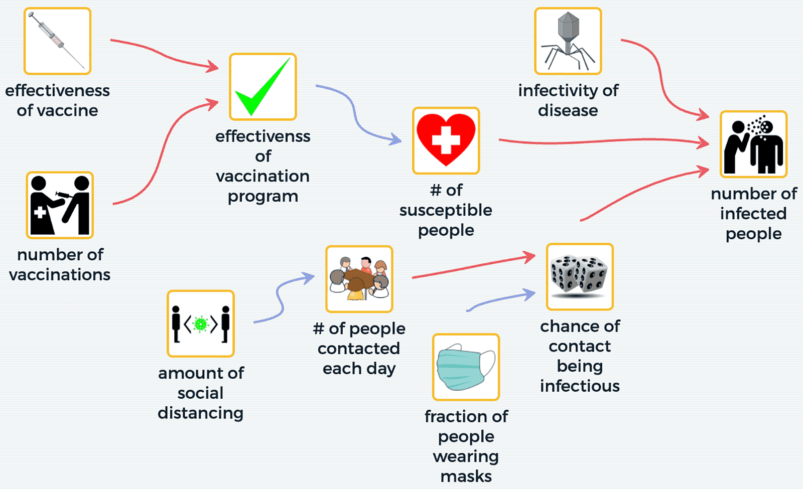
Imagine that you want to create a model to help you determine how bad an epidemic will be based on several factors. In a static equilibrium approach, you first identify the elements of the system affecting the number of people who get infected, then define how each variable affects the others. The combination of susceptible people, infectivity of the virus, and infectious contacts behave similar to an algebraic equation, where a change to one variable causes all other variables to respond as defined by the relationship rules among them (Figure 1). With each change of an independent variable, the entire system immediately adjusts to a new static and stable “state.”
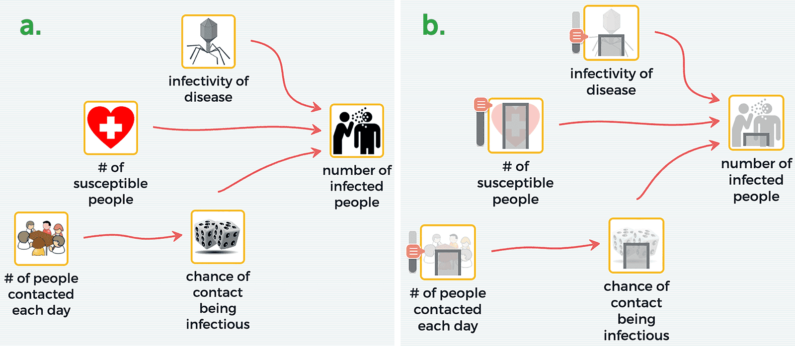
In Figure 1 when # of people contacted each day is increased, a new state of the system is determined by combining this new input value with the other variables in the system, increasing the number of infected people. Each system state results from the set of relationships among the system components, and an adjustment to any of them causes the system to instantaneously reach a new equilibrium. Imagine taking a photograph of the population at one point in time, increasing the number of contacts, and taking another photograph. By comparing the pictures, you can analyze the effect of # of people contacted each day on number of infected people.
Static equilibrium models can be simple or built out indefinitely. For example, we can expand the epidemic model to include variables representing mitigating factors for controlling the epidemic (Figure 2), or expand the boundaries further to consider economic and social impacts. Alternatively, we could include how the virus infects and reproduces at the molecular level.

Dynamic time-based models
Like static equilibrium models, dynamic time-based models in SageModeler represent variables and connections, but with one important additional feature: the ability to represent change over time.
Let’s revisit the epidemic example. Rather than modeling the overall severity of the epidemic, we may want to model how many people will get sick as the epidemic unfolds over time. This was particularly important during the COVID-19 pandemic in order to plan for expanding hospital capacity and to decide when to ease lockdown conditions.
To see an evolution of the model state over time, dynamic models include new kinds of variables—collectors, which can be added to or subtracted from during each model calculation cycle, and flows, which define the rate of change in the collectors (how much is added to or subtracted from the collectors each cycle).
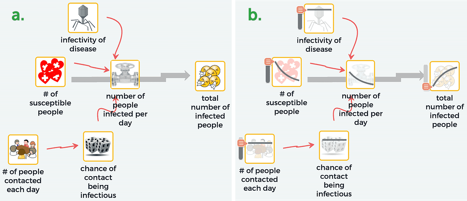
In Figure 3, the # of susceptible people is a collector, as is the total number of infected people variable. The number of people infected per day variable represents how many people become sick during each cycle of the model, causing that number to be subtracted from the # of susceptible people and added to the total number of infected people. This flow, represented as a valve, controls the rate of transfer between the two collectors. Other variables like chance of contact being infectious, infectivity of disease, and # of susceptible people all affect the number of people infected per day. Over time the # of susceptible people decreases and the total number of infected people increases. However, we can see the number of people infected per day starts high and slows down over time (Figure 3b), due to the fact that there are fewer and fewer susceptible people over time to get infected.
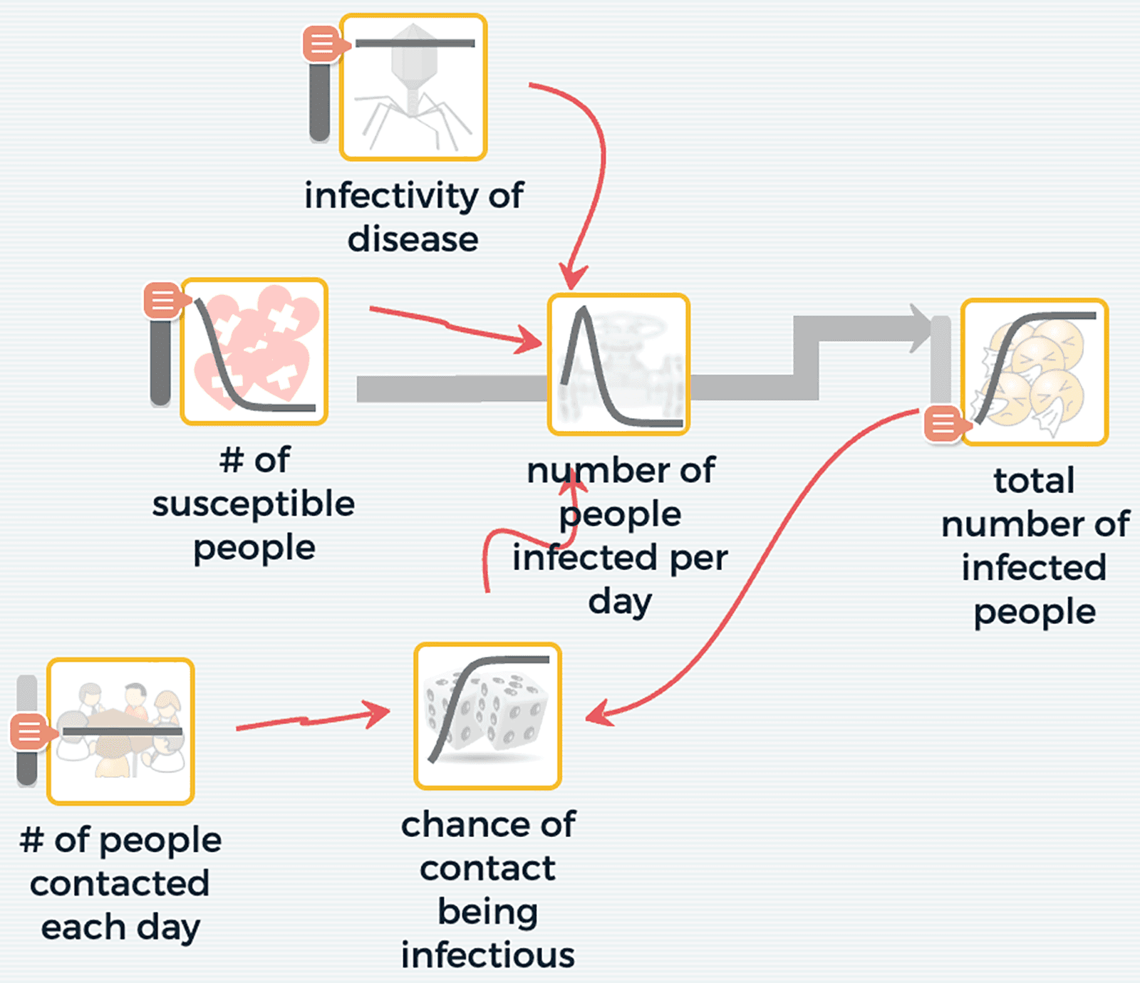
Because collectors can only be added to or subtracted from, they have a “memory” of the system’s state. As such, collectors make it possible for dynamic time-based models to show how feedback causes the system to influence itself. When chains of causal connections loop back upon themselves, the state of a system at one moment can provide the impetus for change into the next. In such a feedback loop, the computer first determines the model state at a given moment by noting the values of all the collectors. These values influence other system variables based on relationship rules that have been set by the student, and eventually, through a chain of cause-and-effect relationships, loop back to influence a variable that is directly connected to the collector that initiated the loop.
In Figure 4, an additional relationship has been defined between the total number of infected people and chance of contact being infectious. This connects to number of people infected per day and back to total number of infected people. Notice how the number of people infected per day more correctly shows the pattern we observed in the real world, when infections start slowly, reach a peak, and then taper off.
Let’s look at another example—this one part of an ecosystem with deer—with two feedback loops (Figure 5). When calculating how the model will behave from moment to moment, we can start with the collector—adult (breeding) deer pop [population]. Tracing the “Reinforcing/positive feedback loop,” the number of adult (breeding) deer in the population directly influences the # new deer births per year, which are added to the number of young deer. The # deer surviving to adult each year are subtracted from the young deer and added to the adult (breeding) deer, completing the feedback loop. In this case, the adult deer population influences the number of new births, adding more young deer to the population, some of which become additional breeding adults. This loop alone would cause the deer population to grow exponentially.

A second loop defines a “Balancing/negative feedback” cycle. In this part of the system the adult (breeding) deer pop is connected to food resources per deer such that an increase in adult deer (breeding) pop causes a decrease in food resources per deer, which eventually impacts the # deer surviving to adult each year added to population. This loop balances out the system so that it can’t grow unchecked.
What type of model should be used?
Before deciding on the modeling approach, it is critical to clarify the model’s purpose. Ask yourself, “What do I want my students to learn by building this model?” If the priority is to analyze the structure and interconnection among components in a complicated system and how a change to a system input affects other system components, static equilibrium modeling may be best.
If it is important to investigate why a particular behavior over time is observed or how a change to a variable alters the way a system develops over time, dynamic time-based modeling is the way to go. Dynamic time-based models allow students to explore feedback-induced behavioral patterns like exponential growth, growth (or decline) to a limit, S-shaped growth, and oscillations.
Both modeling approaches in SageModeler offer students the ability to test their understanding of the system as a whole. Building, revising, and sharing models provides powerful learning opportunities.
Dan Damelin (ddamelin@concord.org) is a senior scientist.
Steve Roderick (sroderick@concord.org) is a curriculum developer.
This material is based upon work supported by the National Science Foundation under grant DRL-1842035. Any opinions, findings, and conclusions or recommendations expressed in this material are those of the author(s) and do not necessarily reflect the views of the National Science Foundation.