Under the Hood: Using WebGL to Accelerate Advanced Physics Simulations in the Browser

Until recently, the idea of running advanced physics simulations in a Web browser was far fetched. While modern Web browsers have 10 times the computational capacity and speed compared with just 18 months ago, pure JavaScript performance isn’t enough for advanced physics. Thanks to the rapid advancement of Web technologies—and a bit of ingenuity—we’re looking past JavaScript and making use of the power of modern GPUs.

WebGL is a powerful part of the new HTML5 standard, bringing graphics card capabilities directly to the browser. WebGL is an implementation of the OpenGL ES 2.0 API in JavaScript, but rendering 3D graphics isn’t the only application of this technology. We’re taking advantage of the GPU computational capacity to speed up physics simulations.

We parallelized the computational fluid dynamics algorithms of our Energy2D simulator and implemented these algorithms using WebGL-based resources. The results are promising. A GPU-enabled simulation is 2-15 times faster than the pure JavaScript implementation!

The most important thing to understand is the difference between CPU and GPU workflow. The graphics processor has enormous computational power, but only if it can do a lot of simple tasks in parallel. GPU doesn’t like complicated routines, like loops or if-else statements. It works fastest when a large number of threads can perform literally identical instructions.

While native applications have access to technologies like CUDA or OpenCL, which provide a high-level interface for parallel programming, these technologies are not (yet) available in the browser. To get WebGL to perform physics calculations, simply trick your graphics processor by pretending that you’re rendering graphics.

First, keep the simulation data in the graphics card memory. WebGL defines 2D texture type. Think of it as an image (or a matrix) with four color channels: R, G, B, A. Each can hold your data and each is encoded using one unsigned byte (accepted values are from 0 to 255). Since this isn’t enough for advanced physics, use OES_texture_float extension, which changes encoding of channels from byte to a 32-bit floating point number.

Next, change the rendering output. By default, what is rendered by the graphics card is displayed on the screen. Fortunately, WebGL allows us to change the render target to the given texture, so we can render directly to our “simulation grid.”

Finally, program the graphics processor with simulation routines and begin rendering. It’s common to render a full-screen quad object to enforce coverage of the whole output texture.

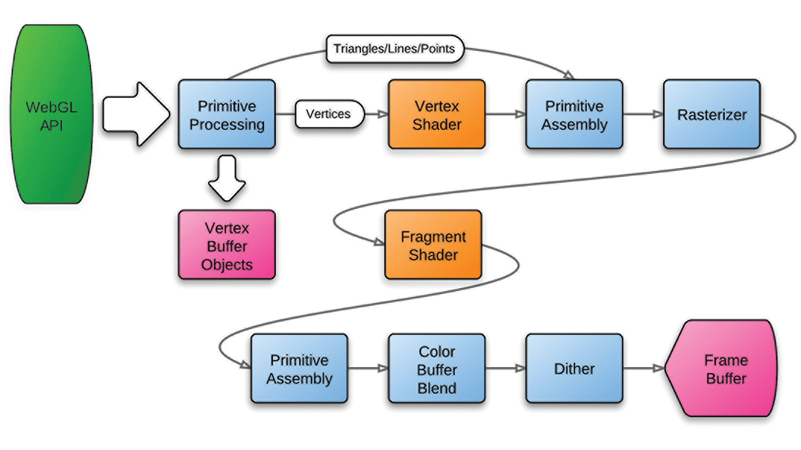
In a typical rendering pipeline, two areas (orange in Figure 1) can be customized using the GLSL language, which has very similar syntax to C.

The Vertex Shader is responsible for transformations of geometry vertices. It’s great when dealing with the perspective and movement or rotation of objects, but it’s often useless for GPGPU calculations.

The Fragment Shader does all the work. GPU executes it for every pixel of output image after geometry rasterization to calculate resulting colors, which can be used for amazing visual effects during graphics rendering. When you’re doing GPGPU calculations, put your routines here. Don’t think about colors, just calculate a new value of a simulation cell represented by a texture pixel. You’ve successfully tricked the GPU!

Piotr Janik (janikpiotrek@gmail.com) was a 2012 Google Summer of Code student for the Concord Consortium.

This material is based upon work supported by Google.org.